WGSA2 Pipeline (updated Jul 2023)
Introduction
The exploration of the microbiome has gained significant attention, leading to the development of powerful computational tools and online pipelines. These tools relieve researchers from the burdensome task of bioinformatics processing for their metagenomics data. Some existing tools (e.g. MetaPhlAn) enable the extraction of taxonomic and functional information directly from shotgun metagenomic short reads. However, more comprehensive analysis, require longer contiguous sequences (e.g. KEGG tools, BLASTp). Unfortunately, there is a scarcity of online tools that provide researchers with computational resources and a command line-free experience to assemble short-read metagenomic datasets for deeper exploration.
To address this computational gap, our Nephele2 team at NIAID designed, developed, and integrated a command line-free Whole Metagenome Sequencing Assembly-based pipeline called WGSA2, into our cloud-based microbiome analysis platform, Nephele. WGSA2 facilitates the processing of shotgun datasets derived from complex microbial communities and diverse habitats, including both host-associated and environmental samples. It generates visualizations and summarized output based on functional and taxonomic annotation, as well as binning of assemblies.
The pipeline offers a user-friendly experience, that omits computational demands and expertise, allows for customizations of profiling strategies and databases (e.g. RefSeq, MGBC, KEGG, MetaCyc). It enables efficient acquisition of biological detail, and grants users with easy access to assembly-based sequences and analysis of their datasets. Overall, WGSA2 fills a computational void in metagenomics, enhances accessibility and comprehension of the data, and paves the way for deeper exploration of the microbiome.
Please visit our online WGSA2 workflow tutorial at WGSA2 workflow - a tutorial
Prerequisites for WGSA2 submission
1. Sequencing data
The input sequences must be paired-end (PE), whole metagenome shotgun reads (not merged) in FASTQ format (see our FAQ on PE vs SE reads). Due to the scaffold-based approach of the assemblies, single-end (SE) reads are not acceptable for WGSA2 pipeline.
2. File formats and dataset size limitations
- WGSA2 can accept both gzipped (.fastq.gz) and unzipped FASTQ files (bam, fasta or other file formats not accepted)
- File names should not contain special characters
- Due to the huge resource and time requirements of WGSA2, which grows with dataset size, the entire sumitted dataset must not exceed 150Gb gzipped. If your dataset exceed this size, please consider splitting it into separate submissions.
3. QC and pre-processing
Datasets submitted to WGSA2 must firstly be run through Nephele's QC pipeline. This pipeline performs basic quality checks, trimming and filtering of the dataset, averts PE mismatch and other issues that can cause failure of WGSA2 (or other) time & resource consuming pipelines. This also helps with troubleshooting potential errors with WGSA2 or other pipelines. Finally the produced QC reports, aids the user to better understand the quality, quantity, size and issues of their samples, sequences and dataset.
4. Mapping file
A metadata file is required during submission of any dataset to the WGSA2 pipeline. This is a tab-delimited file containing information about submitted samples (sample names), the names of their respective FASTQ files, and simple grouping column (called "TreatmentGroup") that provides grouping information for dataset stats and visualization steps. It is advised such file is prepared before submission. The template can be downloaded here. Mapping file can be an .xlsx file or a simple .txt file with the following format:
| #SampleID | ForwardFastqFile | ReverseFastqFile | TreatmentGroup |
|---|---|---|---|
| SampName1 | SampName1_R1.fastq.gz | SampName1_R2.fastq.gz | Control |
| SampName2 | SampName2_R1.fastq.gz | SampName2_R2.fastq.gz | Control |
| SampName3 | SampName3_R1.fastq.gz | SampName3_R2.fastq.gz | Treatment |
| SampName4 | SampName4_R1.fastq.gz | SampName4_R2.fastq.gz | Treatment |
5. Biological considerations
- metagenomic datasets: The WGSA2 pipeline is optimized for shotgun metagenomic datasets only. For other datasets (single organisms, cDNA, etc) the pipeline may hang, fail or process indefinitely. Also, please be advised that some inaccuracies may be produced, depending on phylogenic composition and genetic architecture of some microbial organisms (e.g. in meta-transcriptomic datasets with high ITS content or non-continuous genes) which can produce miss-assemblies or pipeline failures.
- phylogenic composition and community complexity: The WGSA2 pipeline can handle phylogenically diverse communities of single-cell microbial organisms including prokaryotes, viruses and unicellular eukaryotes (e.g. protozoa, single cell fungus, some diatoms). However, currently, WGSA2 is not optimized for identifying complex eukaryotic genes e(splice alternatives).
6. Data upload
There are multiple ways to upload large datasets to Nephele. It is recommended to prepare a Globus end point prior to submission (Tutorial)
Text abbreviations
- TEDreads : reads that have been trimmd & filtered (T), error-corrected (E) and decontaminated (D)
- iTPM: designates the abundance score for each instance of a gene/transcript/annotation
- geneTPM: designates the abundance score for each unique gene / annotation label
- AMR: antimicrobial resistance
- MAGs : metagenome-assembled genomes
User options & electives during submission
1. Run additional trim & filter (elective)
The WGSA2 workflow incorporates a default procedure for baseline trimming and filtering of datasets, ensuring that the dataset meets the basic QA requirements for assembly. Although these settings are sufficient for reliable analysis, users have the option to customize/increase the read trimming and filtration criteria in preparation for assembly processing. This includes the ability to set thresholds for the average quality of reads, trimming the 5' and 3' ends, and/or specify a customized minimum read length.
2. Host Decontamination DB (options)
Given the nature of library preparation and shotgun sequencing, it is necessary to perform decontamination of metagenomic datasets, which allows fore removal of reads that contain any host genomes or biologically uninformative repeat sequences. For this purpose, we have created custom decontamination databases, each tailored to target specific group of host genomes. A detailed description of the content of each custom database is provided below. If you have any uncertainty regarding the appropriate database selection or if you would like to provide feedback and recommendations for such databases for future updates of WGSA2, please don't hesitate to contact the Nephele team.
- Human & Mouse decontamination DB (default choice)
- Description: Human and Mouse hosts
- Content report
- collected assemblies:
- Homo sapiens (assembly version GRCh38.p13),
- Mus musculus (assembly version GRCm39)
- Marine decontamination DB
- Description: Human + 18 common marine host organisms
- Content report
- collected assemblies:
- Homo sapiens (GRCh38.p13),
- Conus ventricosus (ASM1839881v1),
- Crassostrea virginica (C_virginica-3.0) ,
- Crassostrea gigas (cgigas_uk_roslin_v1),
- Mytilus galloprovincialis (MGAL_10),
- Octopus sinensis (ASM634580v1),
- Paraescarpia echinospica (HKBU_Pec_v1),
- Streblospio benedicti (ASM1909598v1),
- Hyalella azteca (Hazt_2.0.2),
- Amphibalanus amphitrite (NRLGWU_Aamphi_draft),
- Paramacrobiotus sp. TYO (Prichtersi_v1.0),
- Hypsibius dujardini (ASM157998v1),
- Lytechinus pictus (UCSD_Lpic_2.0),
- Strongylocentrotus purpuratus (Spur_5.0),
- Apostichopus parvimensis (Ppar_1.0),
- Hydra vulgaris (Hydra_105_v3),
- Hydra viridissima (ASM1470644v1),
- Pocillopora damicornis (ASM370409v1),
- Amphimedon queenslandica (assembly v1.0)
- Mosquito decontamination DB
- Description: Human + 2 common mosquito species
- Content report
- collected assemblies:
- Homo sapiens (GRCh38.p13),
- Aedes aegypti (AaegL5.0),
- Culex quinquefasciatus (VPISU_Cqui_1.0_pri_paternal)
- Nematode decontamination DB
- Description: Human + 15 nematode host organisms
- Content report
- collected assemblies:
- Homo sapiens (GRCh38.p13),
- Caenorhabditis inopinata (Sp34_v7),
- Caenorhabditis nigoni (nigoni.pc_2016.07.14),
- Caenorhabditis elegans (WBcel235),
- Caenorhabditis briggsae (CB4),
- Caenorhabditis tropicalis (Ctrp_NIC203),
- Oscheius tipulae (ASM1342590v1),
- Pristionchus pacificus (El Paco v. 4),
- Ascaris suum (ASM1343314v1),
- Brugia pahangi (ASM1207055v1),
- Steinernema carpocapsae (ASM75764v3),
- Strongyloides ratti (S_ratti_ED321),
- Heterodera glycines (ASM414822v2),
- Haemonchus contortus (haemonchus_contortus_MHCO3ISE_4.0),
- Trichinella spiralis (Trichinella spiralis-3.7.1),
- Trichinella murrelli (ASM222148v1)
- Rodent decontamination DB NEW
- Description: Mouse + 5 other rodents
- Content report
- collected assemblies:
- Homo sapiens (assembly version GRCh38.p14),
- Mesocricetus auratus (BCM_Maur_2.0 and MesAur1.0),
- Mustela putorius furo (ASM1176430v1.1),
- Mustela nigripes (MUSNIG.SB6536),
- Mustela erminea (mMusErm1.Pri),
- Mustela nivalis (MusNiv_Pri1.0),
- Mus musculus (GRCm39),
- Mus caroli ( CAROLI_EIJ_v1.1),
- Mus pahari (PAHARI_EIJ_v1.1)
- Primates decontamination DB NEW
- Description: Common primate host organisms + human
- Content report
- collected assemblies:
- Homo sapiens (assembly version GRCh38.p14),
- Macaca mulatta (Mmul_10),
- Macaca fascicularis (MFA1912RKSv2),
- Macaca nemestrina (Mnem_1.0),
- Cercocebus atys (Caty_1.0),
- Pan troglodytes (NHGRI_mPanTro3-v1.1-hic.freeze_pri),
- Pan paniscus (NHGRI_mPanPan1-v1.1-0.1.freeze_pri),
- Gorilla gorilla (NHGRI_mGorGor1-v1.1-0.2.freeze_pri),
- Pongo pygmaeus (NHGRI_mPonPyg2-v1.1-hic.freeze_pri),
- Callithrix jacchus (mCalJa1.2.pat.X)
- Plants decontamination DB NEW
- Description: Standard reference DB of ~111 plant host organisms from RefSeq
- Content report
- collected assemblies: RefSeq complete plant genomes
3. TAX classification DB (options)
WGSA2 can now provide users with an option to elect the best taxonomic classification database to fit their dataset's needs. Options are:
- Kraken2 Standard Reference Genomes DB (kr2_RefDB) [default]::
- Description: ~15K reference genomes from Bacteria, Archaea, Viruses and single-cell eukaryotic Protozoa & Fungi. This database is the optimal choice for datasets of unknown community complexity and richness.
- Info: Source. Build: March, 2023
- Content report
- Mouse Bacterial Gut Catalogue DB (MGBCDB):
- Description: The genomes of >26.6K prokaryotic organisms characteristic for mouse gut microbiomes. Not all genomes contained within this DB are reference genomes.
- Info: Source, Build: May 2021
- Content report
- Eukaryotic Pathogens DB (EuPathDB):
- Description: known eukaryotic pathogen detection (no prokaryotic organisms).
- Info: Source. Build: April 2023
- Content report
4. Output downloadable TEDread fastq files (elective)
After the baseline QA and decontamination steps, the pipeline generates TEDreads (trimmed, filtered (T), error-corrected (E), and host-decontaminated (D) reads) for each sample. The size of these files can be quite large, depending on the level of host contamination and the quality of the reads. Including these files as part of the results of the pipeline significantly increases the already bulky output. Hence, we have made the decision to remove them from the default pipeline output, and provide them as an optional separate download link. Electing this option, will provide this link in the results page after pipeline completion.
5. Run AMR finding (elective)
For users that are interested in the Antimicrobial Resistance Peptides (AMRs) content of their samples, we have provided an elective option to run AMRFidnderPlus on the assembled genes for each sample. Since this additional step is resource and time consuming, it is omitted from the default workflow of the pipeline. Please be aware that by selecting this option, adding additional compute time will be required for the completion of the pipeline.
6. Metabolic pathways database (options)
Functional capacity of a community is assessed by mapping the gene annotations from each sample against a database of known functional pathways. WGSA2 provides the user with 2 choices of functional pathway databases - the KEGG DB (as of Sept 2022), which uses KO annotations [default], or the MetaCyc DB (as of Sept 2022), which utilizes the EC annotations of the dataset. There is no wrong choice.
7. Produce gene-based or scaffold-based taxonomic profiles (electives)
As a default setting, WGSA2 utilizes the Kraken2 tool (refer to Workflow section Step 3) to generate taxonomic profiles based on TEDreads for each sample. Through extensive testing, we have found these Kraken2 profiles to be highly accurate, taxonomically sensitive, and computationally lenient. Additionally, users have the option to generate taxonomic characterizations on the predicted genes (or scaffolds) within each sample, which also allows for the evaluation of community profiles. While these alternative approaches may have lower sensitivity in detecting taxonomic presence and abundance, they are valuable for identifying genes (or genomic regions) associated with specific organisms of interest. Please note that utilizing alternative or multiple TAX profiling strategies is necessary, for reliable taxonomic characterization of a dataset and would generally produce concordant results. Therefore, Gene and Scaffold-based profiles are not part of the default pipeline output.
8. Produce MAGs (elective)
This option enables the generation of metagenome-assembled genomes (MAGs) and is optimized for communities with known and prokaryote-rich organisms, catering to users interested in the more abundant organisms within their samples. It's important to note that this option of the WGSA2 pipeline is highly resource and time-consuming, which may result in increased job-time. It is advisable to use subsets of selected samples when utilizing this option. Despite the reduced resolution at the community level, the MAG-based taxonomic profiles generated by this WGSA2 option are highly accurate and can provide detailed strain-level information.
Workflow
Note: Click to the diagram to zoom in/out
Steps 1 & 2: Trimming, Error-correction and Decontamination (TED)
The WGSA2 pipeline begins by processing reads in preparation for assembly, which includes 3 steps (process acronym is chosen as TED):
- (T) trimming and filtering of reads (fastp). This step is not as thorough as the recommended pre-processing performed by our QC pipeline and therefore should not be considered its replacement. By default, this step verifies that the reads have met the required minimal QA standards. However, if the user desires to apply more stringent quality thresholds after running the QA pipeline, this step allows for such customization through elective trimming and filtering options. (see user options section)
- (E) error-correction (fastp). PE sequences are merged and sequencing errors are corrected within the PE overlapping regions. This process is specifically designed to improve assembly efficiency and success.
- (D) decontamination (Kraken 2). The dataset undergoes a thorough cleaning process to remove host DNA and non-informative elements such as homopolymeric or simple sequence repeats. This is achieved by utilizing a user-selected database containing curated collections of potential host organism genomes (see user options section). The decontamination process is crucial for reducing the dataset size to include only biologically relevant data. By removing non-informative host, junk and repeat sequences, the assembly quality is significantly improved for each sample. Contamination levels and identification of host organisms are reported per sample in the form of \$SampleName_decontamREPORT.
Step 3: TAX profiling
By default, WGSA2 includes the generation of taxonomic profiles per sample based on the TED reads, utilizing the Kraken 2 tool. Our tests have demonstrated that Kraken 2 is a computationally efficient method that provides moderate accuracy and taxonomic sensitivity compared to other common profiling methods (e.g., gene-based or alternative tools). Kraken relies on a comprehensive database of k-mers derived from entire genomes, enabling accurate taxonomy assignment for both coding and non-coding reads. WGSA2 offers users the flexibility to choose the classification databases that best suit their datasets (see user options section). The resulting taxonomic profiles are visualized using the Krona tool on a per-sample basis, and they are also consolidated into a summary community matrix table (see Step 9). This table serves as a foundation for customized project-specific community analysis by the user, while WGSA2 additionally provides basic statistics and visualizations in steps 10-11.
Steps 4 & 5: de novo assembly, read mapping and abundance scoring
In this step, the pipeline uses metaSPAdes assembler, to perform de novo assembly of the TED reads. The process is performed for each sample independently.
Next, Bowtie2 and SAMtools are used to align each sample's TED reads to the sample's assembly (a process called 'mapping'). The alignment is also QC'd and cleaned (de-replicated, mate pairs are fixed, etc) to ensure each pair of reads maps best and only once to the produced assembly. Then, the aligned reads are evaluated (GC content, plus/minus strand alignments), enumerated and abundance scores produced per scaffold per sample (scaffold length, depths, coverage, RPM (reads per million), etc. statistics are collected). This information is used for downstream abundance assessments.
Note: this is one of the most time & resource consuming stages of the pipeline and depending on sample size may take longer than a few hours per sample. Parallelization is used to achieve assembly of multiple samples simultaneously (however patience is still required). Pipeline failures in this processing stage suggests problematic sample depths or read quality.
Steps 6 & 7: Gene prediction & annotation
WGSA2 utilizes Prodigal for performing genetic feature predictions, and EggNOG-mapper2 against the extensive EggNOG-v5 database for annotation of the predicted features. Gene annotations produced are based on KO, EC and COG annotation terms.
Gene abundance scores are computed by enumerating the number of reads aligned to the gene coordinates of the scaffold (VERSE tool)(used: default settings "featureCounts", -z 0). RPM and TPM (transcripts per million) values are calculated based per transcript instance in each scaffold per sample and produce the abundance scores of each gene (iTPM).
NEW Since each sample contains multiple organisms that may contain multiple copies of any given gene transcript, gene abundances are also summarized per unique gene annotation in each sample (geneTPM). A geneTPM abundance matrix is now provided with WGSA2
Step 8: Pathway inference
Based on the user's chosen option for functional database (KEGG or MetaCyc), the functional profiles for each sample is generated by mapping the the corresponding gene annotation terms (KO or EC) to their corresponding database of pathways. This mapping is accomplished by MinPath, which is a parsimony approach for reconstructing the minimal set of pathways described by a query of genes. The abundance of each pathway is then calculated by averaging the iTPM values (from each instance of gene) from each gene within each inferred pathway. To achieve this, the script 'genes.to.kronaTable.py' is employed. The resulting functional profiles, representing metabolic pathway profiles, are summarized for each sample in an HTML file using KronaTools.
Steps 9: Dataset collations & abundance matrix summaries
These steps are conditional to datasets containing multiple samples (best if >3 samples). Firstly, the community profiles from each sample are collated to create 1 abundance matrix per profile type, which represents the dataset. These profile types producing community matrices are:
- per Taxonomic composition for each sample (unique species composition)
- per Genetic composition for each sample (unique gene composition)
- per Functional composition for each sample (inferred pathway composition)
The Taxonomic and Functional profile matrices are further formatted into biom files that include metadata. These biom files can be conveniently uploaded into MicrobiomeDB or customized for other user-specific purposes.
Step 10: Community visualizations and summaries
The created abundance matrices are imported in R to produce simple community characterizing visualization plots (e.g. alpha and beta diversity plots, abundance profile heat-maps etc.).
Workflow: add-ons
In addition to the main workflow of WGSA2, the user has a few additional options for consideration. Those include:
- Creation and evaluation of MAGs
- Production of gene or scaffold taxonomic assignments (depending on research interest)
- AMR gene finding
Creation and evaluation of MAGs
Users have the option to select the MAGs (metagenome-assembled genomes) feature in WGSA2, which enables the generation of individual genomes from metagenomic assemblies. The WGSA2 pipeline employs MetaBat2 to bin scaffolds with a length greater than 1500bp, based on scaffold features like connectivity, GC content and read coverage. This process aims to reconstruct the most representative genomes of each community. Quality assessments of the resulting MAGs are performed using CheckM. The assessment includes taxonomic affiliation, MAG size, abundance estimations, completeness, contamination levels, number of genes, and more. Additionally, a biom file is generated, consolidating the MAGs data from all the samples.
Please note that the MAGs option within WGSA2 is primarily recommended for prokaryotic-dominated communities, as the classification of eukaryotic draft genomes (bins) may not be as accurate. Taxonomic profiles are once again produced, summarized, and visualized per sample using KronaTools. While MAG-based profiles align closely with TEDread-based profiles, they may be less sensitive in capturing less abundant organisms (for more details, refer to WGSA2 benchmarking section).
Production of gene or scaffold based taxonomic profiles
By default, WGSA2 will produce TEDread-based taxonomic profiling with Kraken2. User may elect to additionally produce taxonomic characterization of the predicted features or scaffolds, within each sample, and community profiles based on those classifications. These can be useful in identifying genes (or genomic regions) within specific taxonomies of interest. WGSA2 will utilize the same classification database for gene or scaffold profiling, as elected for the TEDread-based taxonomic profiling.
AMR gene finding
User may elect to run the antimicrobial resistance gene tool AMRFinderPlus using the predicted features from each sample. This option is time consuming and not provided in the default output.
Pipeline output details
Please refer to this file for the complete and detailed list of the pipeline output & details. File will also be part of the main output downloaded from the pipeline. Here, we detail only the outputs of the main result aggregate folders
TAXprofiles folder
Contains dataset-wide taxonomic results
Although listed first here, this folder is one of the last produced from the pipeline as it contains the dataset-wide taxonomic results (visualizations, summaries and community matrices) produced from each processed sample.
Complete contents of this folder will depend on the options elected for the pipeline.
readsTAX_<DBname>folder (default): Contains logs and reports from the taxonomic classification of TED reads. Sub-folders:binfolder: files used by Krona for creating theTAXplotshtml chart. These are the text versions of the per-sample taxonomic reports from the TED reads, and they are visualized in theTAXplots_ReadsTAX_<DBname>.htmlreport.biomsfolder: The files from thebinfolder presented in a json biom format. These can be manually uploaded to MicrobiomeDB or any other analytical platform, if needed.reportsfolder: contains Kraken2 report files with detailed taxonomic classifications produced for each sampleTAXplots_readsTAX_<DBname>.htmlfile: interactive Krona chart of the TED read-based taxonomic profiles, collected in thebinfolder.merged_tablesfolder (conditional of ≥ 2 samples): a folder containing the collated taxonomic abundance matrix from the entire dataset. The TAX abundance matrix is reported in 6 tab-delimited text files and 1 biom file. The files are named based on content and format of certain profile information: TAX-labels designate files that contain the taxonomy in separate columns per rank, the Lineage-labels designate files representing the lineage of each taxonomy (all tax ranks) in 1 column (ranks separated by ';' within the column). Counts-label indicates files representing the abundance counts of each taxonomy for each sample (collated across dataset). The biom file represents counts for each sample and lineage column. This is the source file for thefor_analyze_with_microbiomedb.biomin main folder.DivPlotsfolder (conditional of ≥ 2 samples): Diversity plots and exploratory statistics for the dataset (note new location is withinReadsTAXfolder as it summarizes the data from the ReadTAX profiles). The plots include alpha diversity indices table and boxplot (TAX_AlphaDiv.txtandTAX_AlphaDiv.pdf), beta diversity PCoA and nMDS ordination plots (TAX_BetaDiv_nMDS.pdf&TAX_BetaDiv_PCoA.pdf, require >=3 samples), TAX content heatmap (TAX_Profile_Heatmap.pdf), Rank Abundance Curve plot (TAX_RankAbundanceCurve.pdf) and Rarefaction Curves (TAX_RarefactionCurve.pdf). In some cases (e.g. ordination plots), some exploratory statistics will fail due to the content of the dataset.
geneTAX_<DBname>folder (based on user-elections): Conditional on the choice of classification DB, visual summary of the gene-based taxonomic annotations for each sample, are presented here. Note: MGBCdb does not produce visual summaries. This folder contains abinfolder with text versions of the profiles from each sample and aTAXplots_genetax.htmlinteractive krona plot summary file of the gene-based taxonomic profiles from each sample.MAGs_TAXfolder (based on user-elective): This folder is generated only if MAGs creation and taxonomic profiling is enabled. It contains the TAX classification and abundances of the MAGs. It also contains abinfolder with text versions of the MAG-based taxonomic profiles and visualizations by KronaTools (TAXplots_MAGx.html). It will also contain aMAG-based_Counts+TAX.biomfile summarizing the MAG-based taxonomic profiles of all samples.
Note: scaffold-based taxonomic annotations option will not produce visualizations, but annotations are reported within each sample's assembly folder.
PWYprofiles folder
Contains dataset-wide functional results
Contains dataset-wide the functional analysis results from the pipeline, including pathway inferred profiles (PWY) and gene-based profiles. The folder will contain one folder, named based on the metabolic pathway database chosen at submission: keggPWYs.MP (default choice) or metacycPWYs.MP (alternative choice). Either folder will have the same structure:
PWYplots_[ko2gg or ec2cc].html: an interactive krona html report with the functional profiles for each sample (KronaTools), based on inferred PWYspwybinfolder: per-sample text reports of the PWYs identity & abundances files. the files are used to create the html report & biom filesbiomsfolder: the json biom versions of the pwybin files.genebinfolder NEW : per-sample text reports of identity and abundances of each unique gene found in the sample.merged_tablesfolder (conditional of ≥ 2 samples): Dataset-wide PWY abundance summary abundance matrix tables representing the collated results each sample functional annotation and abundance scoring. The PWY abundance matrix is reported in 6 tab-delimited text files and 1 biom file. The files are named based on content and format of certain profile information: PWY-labels designate files that contain the pathway information as separate columns per tiers, the allTiers-labels designate files representing the Tiers of each pathway in 1 ';'-delimited column. Counts-label indicates files representing the abundance counts of each pathway for each sample (collated across dataset). The biom file represents counts for each sample and tiers column. NOTE: As of the latest WGSA2 update, the folder also contains a NEW file - a gene-based abundance matrix (merged_geneTPMtable.txt) produced from the collated gene abundance information in thegenebinfolder.DivPlotsMP(conditional of ≥ 2 samples): Simple exploratory plots of PWY functional dataset-wide profiles. Visualizations include a community PCoA and nMDS functional composition ordination plots (PWY_BetaDiv_nMDS.pdf&PWY_BetaDiv_PCoA.pdf; (>=3 samples)) produced from the inferred PWY matrix inmerged_tables.MPas well as a pathway abundance heatmap plot (PWY_Profile_Heatmap.pdf(>=2 samples)).
Accuracy of WGSA2 profiling
We sought to assess and benchmark the accuracy of the WGSA2 taxonomic assignments by evaluating results when running the pipeline with known microbial community. For this, we used the 2nd CAMI Toy Human Microbiome Project Dataset (Sczyrba et al. 2017). The plots bellow represent results from the comparison of the taxonomic and functional profiles of 3 CAMI samples (S1-GI, S6-Oral & S28-Skin) against each other, as produced by the various strategies of WGSA2, BioBakery or as expected by sample design. To produce these comparisons, the community abundance matrices from each pipeline and strategy were merged based on TAXid, rarified to same readDepths (sample with lowest read depth) and ASVs filtered at relative abundance >0.5%.
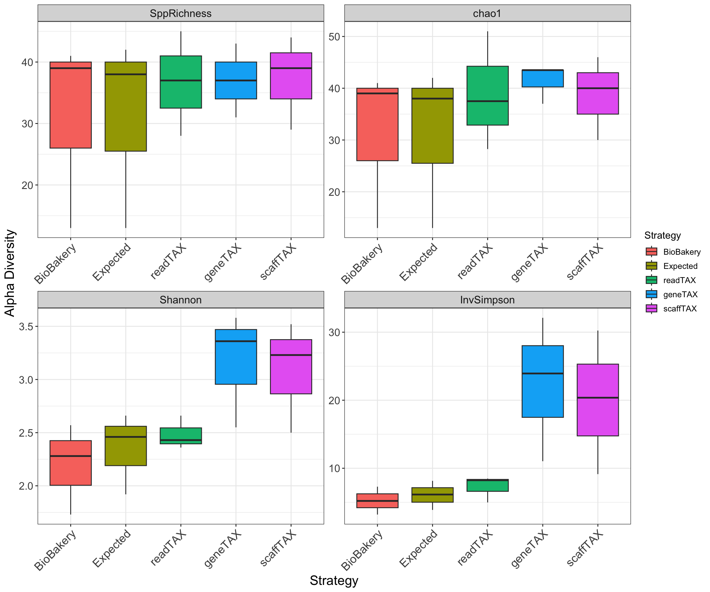
The Alpha Diversity box plots represent the average Shannon diversity & produced Species Richness from the 3 samples. This plot best presents the overall accuracy of the strategies used by WGSA2 TAX assignments. To produce these plots, the community abundance matrices from each strategy were merged based on TAXid, rarified to sample with lowest read depth and filtered to relative abundance of 0.5%.
1) A heatmap of the top 35 species from 3 CAMI sample profiles, produced by the WGSA2 TED-read-based TAX profiles (Kraken2 at confidence level 0.05), the BioBakery pipeline (MetaPhlAn3), and as Expected by sample design).

2) Alpha Diversity box plots, represent the average Species Richness, Chao1, Shannon & InvSimpson Diversity across 3 CAMI samples. The plot demonstrates the overall expected accuracy of the strategies used by WGSA2 for TAX assignments and compares them to the expected profiles and the BioBakery produced TAX profiles
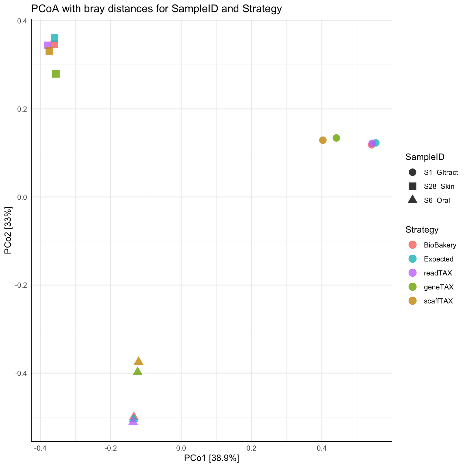
3) Beta Diversity PCoA ordination plot based on Bray-Curtis dissimilarity matrix, produced from 3 CAMI samples from WGSA2 TAX profiles based on different strategies (read, gene & Scaffold-based TAX profiles), BioBakery produced profiles and as expected by design
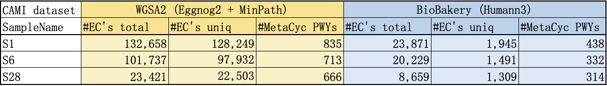
4) A table for number of predicted EC annotations and unique pathways, produced from WGSA2 vs BioBakery
If you wish to test the WGSA2 pipeline, you can find and download a small example dataset (3 CAMI samples, subset to read depth of 1 million reads) and corresponding mapping file specific for the WGSA2 pipeline, from Nephele's User Guide page
Disclaimer
WGSA2 pipeline is optimized for shotgun metagenomic datasets. Although it can be used on metatranscriptomics datasets, some RNA features (e.g. internal transcribed spacer regions (ITS)) might produce miss-assemblies and inaccuracies in the predicted features or their abundance scores. Please avoid using WGSA2 on metatranscriptomics datasets or accept the risk of existing inaccuracies in the produced output.
The Nephele team is working hard to improve and extend this pipeline to provide users with a better experience and more analyses. Please kindly provide us with feedback and keep an eye on Nephele updates.
Software, scripts, tools utilized by the pipeline
Tool versions used by the pipeline are recorded in log file
- fastp
- kraken2
- spades
- bowtie2
- bbtools
- samtools
- MetaBAT 2
- Prodigal
- eggNOG-mapper2
- verse
- AMRFinderPlus
- KronaTools
- MinPath
- R statistical computing
- kreport2krona.py
- CheckM
- biom-format
References
- Angelova AG, et al. (2023). WGSA2 workflow - a tutorial. https://dx.doi.org/10.17504/protocols.io.n92ldm98xl5b/v1
- Joint Genome Institute. BBtools. 2014
- Shifu Chen, Yanqing Zhou, Yaru Chen, Jia Gu, fastp: an ultra-fast all-in-one FASTQ preprocessor, Bioinformatics, Volume 34, Issue 17, 01 September 2018, Pages i884–i890, https://doi.org/10.1093/bioinformatics/bty560
- Bankevich et al. SPAdes: A New Genome Assembly Algorithm and Its Applications to Single-Cell Sequencing. J Comput Biol. 2012 May; 19(5): 455–477.doi: 10.1089/cmb.2012.0021
- Langmead, B., Trapnell, C., Pop, M. et al. Ultrafast and memory-efficient alignment of short DNA sequences to the human genome. Genome Biol, (2009). https://doi.org/10.1186/gb-2009-10-3-r25
- Li H, Handsaker B, Wysoker A, Fennell T, Ruan J, Homer N, Marth G, Abecasis G, Durbin R; 1000 Genome Project Data Processing Subgroup. The Sequence Alignment/Map format and SAMtools. Bioinformatics. 2009 Aug 15;25(16):2078-9. doi: 10.1093/bioinformatics/btp352. Epub 2009 Jun 8. PMID: 19505943; PMCID: PMC2723002.
- Kang, Dongwan D et al. MetaBAT 2: an adaptive binning algorithm for robust and efficient genome reconstruction from metagenome assemblies, PeerJ. 2019, doi:10.7717/peerj.7359
- Cantalapiedra Carlos P., Hernandez-Plaza Ana, Letunic Ivica, Bork Peer, Huerta-Cepas Jaime. eggNOG-mapper v2: functional annotation, orthology assignments, and domain prediction at the metagenomic scale. biorxiv. (2021) doi: https://doi.org/10.1101/2021.06.03.446934
- Hyatt, Doug et al., Prodigal: prokaryotic gene recognition and translation initiation site identification., BMC bioinformatics vol. 11 119. 8 Mar. 2010, doi:10.1186/1471-2105-11-119
- Parks, Donovan H et al., CheckM: assessing the quality of microbial genomes recovered from isolates, single cells, and metagenomes., Genome research vol. 25,7 (2015): 1043-55. doi:10.1101/gr.18607214
- Ondov, B.D., Bergman, N.H. Phillippy, A.M. Interactive metagenomic visualization in a Web browser. BMC Bioinformatics, 385 (2011). https://doi.org/10.1186/1471-2105-12-385
- Ye Y, Doak TG (2009) A Parsimony Approach to Biological Pathway Reconstruction/Inference for Genomes and Metagenomes. PLOS Computational Biology 5(8): e1000465. https://doi.org/10.1371/journal.pcbi.1000465
- Caspi et al 2020, The MetaCyc database of metabolic pathways and enzymes - a 2019 update, Nucleic Acids Research 48(D1):D445-D453
- Zhu, Q., Fisher, S.A., Shallcross, J., Kim, J. (Preprint). VERSE: a versatile and efficient RNA-Seq read counting tool. bioRxiv 053306. doi: http://dx.doi.org/10.1101/053306
- H. Li, Seqtk: a fast and lightweight tool for processing FASTA or FASTQ sequences, 2013.
- Carlos P. Cantalapiedra, Ana Hernandez-Plaza, Ivica Letunic, Peer Bork, and Jaime Huerta-Cepas., eggNOG-mapper v2: functional annotation, orthology assignments, and domain prediction at the metagenomic scale. 2021, Molecular Biology and Evolution, https://doi.org/10.1093/molbev/msab293
- Minoru Kanehisa, Yoko Sato, Masayuki Kawashima, Miho Furumichi, Mao Tanabe, KEGG as a reference resource for gene and protein annotation, Nucleic Acids Research, 2016, https://doi.org/10.1093/nar/gkv1070
- Wood, D.E., Lu, J. & Langmead, B. Improved metagenomic analysis with Kraken 2. Genome Biol, 2019. https://doi.org/10.1186/s13059-019-1891-0
- R Core Team (2021). R: A language and environment for statistical computing. R Foundation for Statistical Computing, Vienna, Austria. URL
Acknowledgments
This pipeline is made possible, public and free due to the efforts of scientists from BCBB Bioinformatics and Computational Biosciences from OCICB/OSMO/OD/NIAID/NIH and the Nephele Team
Contact us
For feedback, questions, problems or concerns with WGSA2, please contact us at nephelesupport@nih.gov, with specific mention of the WGSA2 pipeline in subject. Thank you.